From a TELEMAC 2D model
Preamble
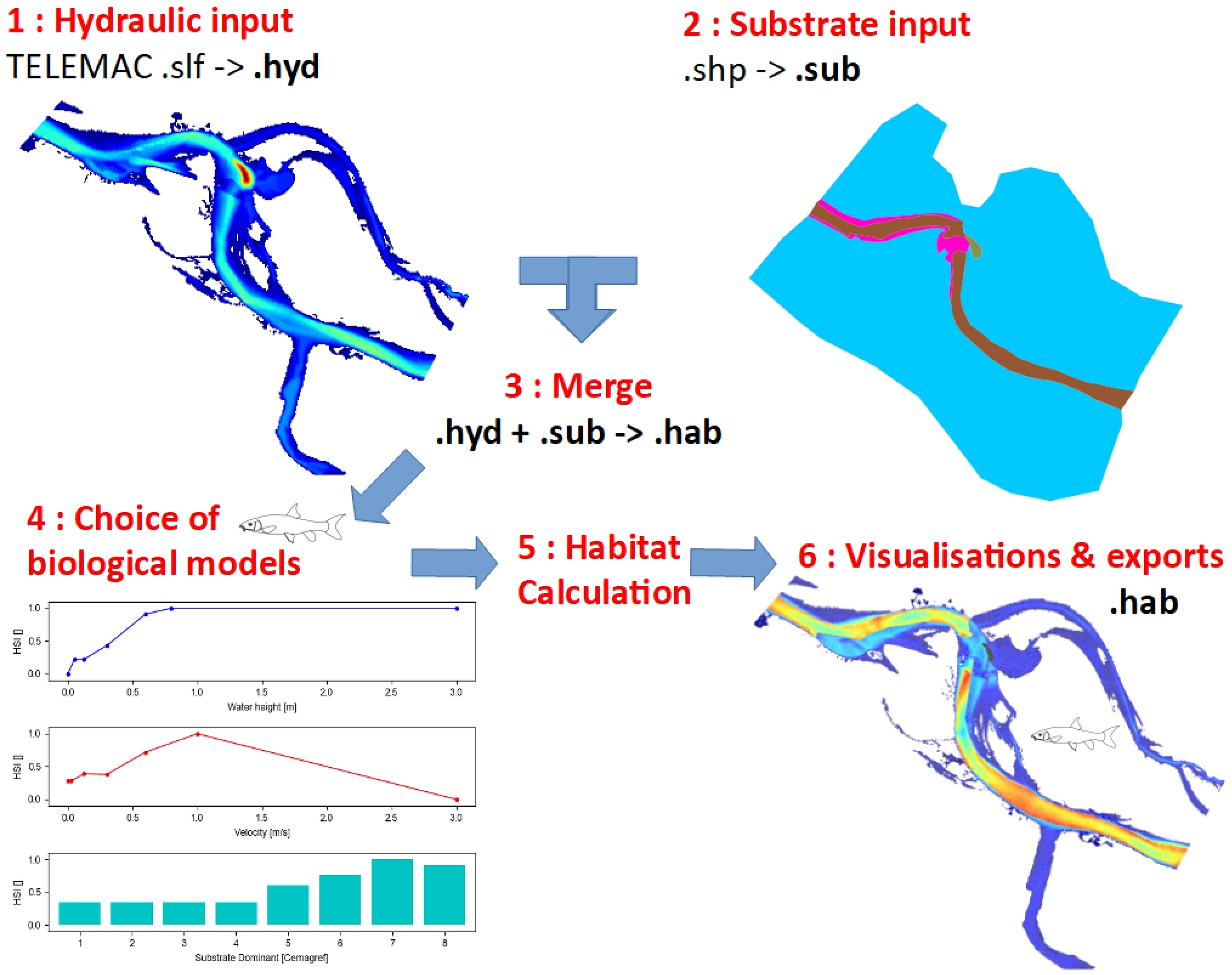
The objective of this tutorial is to model the habitat of the adult barbel from several TELEMAC 2D hydraulic simulations. The results will be visualised in interactive figures, in GIS output and in 3D. The main steps are as follows:
- TELEMAC data will be read by the software to create a hydraulic .hyd file.
- The substrate data will be read by the software to create a .sub substrate file.
- The .hyd and .sub files will be merged into a .hab file from which HABBY can perform habitat calculations.
- The biological model of the adult barbel will be selected.
- The habitat calculation will be performed.
- The results will then be visualised and exported.
Prerequisites
- Install HABBY.
- Download and extract the hydraulic and substrate example files:
- GIS software, such as QGIS or ArcGIS (for viewing map exports).
- The open-source software Paraview (to visualise the 3-dimensional exports) https://www.paraview.org/.
- A spreadsheet program, such as LibreOffice Calc or Excel (for viewing TXT exports).
Description of input files
Hydraulics


| File(s) used | Description |
|---|---|
| d1.slf, d2.slf, d3.slf, d4.slf, d5.slf, d6.slf d7.slf, d8.slf, d9.slf | 2D TELEMAC modelling of a multi-flow braided river. These files are permanent discharge simulation result files. Each file represents a simulated constant discharge. Each file contains a single time step. |
| indexHYDRAU.txt | To use multiple hydraulic input files at the same time in HABBY, it is necessary to have previously created a indexHYDRAU.txt file to assign a discharge value to each input file. |
| discharge_chronicle.txt | This file is used with the HABBY interpolation tool (optional for habitat calculation). |
Here are the contents of the indexHYDRAU.txt file:
EPSG=unknown
filename Q[m3/s]
d1.slf 9.2
d2.slf 21.2
d3.slf 35
d4.slf 48.4
d5.slf 74.7
d6.slf 110
d7.slf 150
d8.slf 175
d9.slf 259
Substrate


| File(s) used | Description |
|---|---|
| sub_PolygonSandreCoarser-dom.shp (and associated files .shx, dbf, ..) | This GIS data is of type Shapefile and represents polygons of homogeneous substrate. Mapping method : Polygon (Polygon). Classification code : Sandre (Malavoi and Souchon 1989). Classification method: coarser-dominant (PlusGros-Dominant). |
| sub_PolygonSandreCoarser-dom.txt | It is necessary to have previously created a file with the same name as the Shapefile, i.e. 'sub_PolygonSandreCoarser-dom.txt' in order to indicate to HABBY the classification code and the classification method of the substrate as well as the default substrate values (in case of not complete superposition of the substrate on the hydraulic). The latter is provided with the example data set. |
Here are the contents of the file 'sub_PolygonSandreCoarser-dom.txt':
substrate_classification_code=Sandre
substrate_classification_method=coarser-dominant
default_values=12, 12
Step by step
Create a new project
- Start the software.
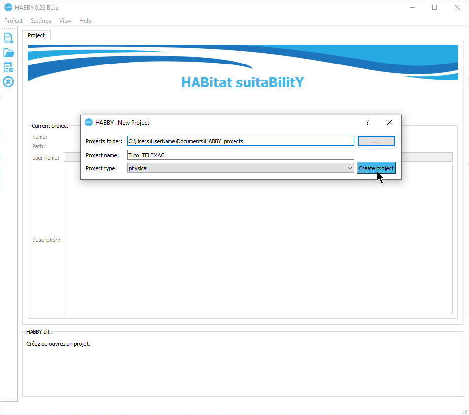
- Go to menu <hi #47B5E6>Project - New</hi>.
This opens the <hi #9BFFFF>HABBY - New Project</hi> window.
- Enter in <hi #9BFFFF>Project name:</hi>: 'Tuto_TELEMAC'.
- Choose in <hi #9BFFFF>Project type:</hi>: 'physique'.
- Click on <hi #47B5E6>[Create Project]</hi>.
The project is then created and gives you access to new tabs.
Creating a .hyd file
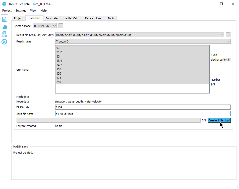
- Open the tab <hi #9BFFFF>Hydraulic</hi>.
- For <hi #9BFFFF>Select a model</hi> choose 'TELEMAC 2D'.
This opens the input file manager for TELEMAC.
- If the pre-reading went well, the software should display the following information:
- <hi #9BFFFF>Reach name:</hi>: 'Tronçon D'.
- <hi #9BFFFF>Unit name:</hi>: selection of '9.2' to '259'
- <hi #9BFFFF>Type</hi>: 'discharge [m3/s]'
- <hi #9BFFFF>Number</hi>: '9/9'
- <hi #9BFFFF>Mesh data</hi>: ''
- <hi #9BFFFF>Node data</hi>: 'elevation, water depth, water velocity'
- <hi #9BFFFF>EPSG code</hi>: '2154'
- <hi #9BFFFF>.hyd filename</hi> : 'd1_to_d9.hyd'
- If this information is valid, you can start the calculation by pressing the <hi #47B5E6>[Create 1 file .hyd]</hi> button.
Once the process is complete, a file 'd1_to_d9.hyd' is created.
Creating a .sub file
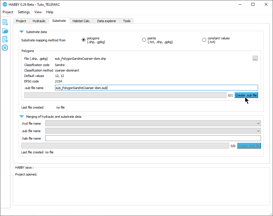
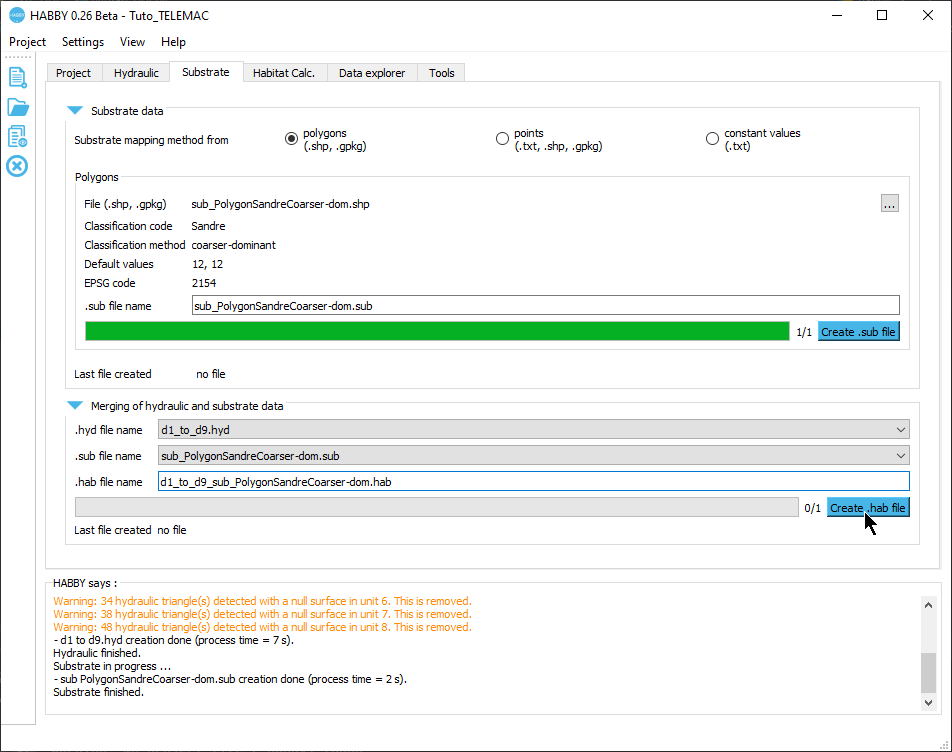
- Open the <hi #9BFFFF>Substrate</hi> tab.
- For <hi #9BFFFF>Substrate mapping method from</hi> check that 'polygons (.shp, .gpkg)' is selected.
- If the pre-reading went well, the software should display the following information:
- <hi #9BFFFF>File (.shp, .gpkg)</hi>: 'sub_PolygonSandreCoarser-dom.shp'
- <hi #9BFFFF>Classification code:</hi>: 'Sandre'
- <hi #9BFFFF>Classification method:</hi> : 'coarser-dominant'
- <hi #9BFFFF>Default values</hi> : '12, 12'
- <hi #9BFFFF>EPSG code</hi>: '2154'
- <hi #9BFFFF>.sub file name</hi> : 'sub_PolygonSandreCoarser-dom.sub'
- If the information displayed in this tab is valid, you can start the calculation by pressing the <hi #47B5E6>[Create .sub file]</hi> button.
Once the process is finished, a file 'sub_PolygonSandreCoarser-dom.sub' is created.
Creating a .hab file
- Stay in the <hi #9BFFFF>Substrate</hi> tab.
- In the <hi #9BFFFF>Merging of hydraulics and substrate data</hi> group, check that the file names are selected for:
- <hi #9BFFFF>.hyd filename</hi>: 'd1_to_d9.hyd'.
- <hi #9BFFFF>.sub filename</hi>: 'sub_PolygonSandreCoarser-dom.sub'.
- Then launch the merge with the <hi #47B5E6>[Create .hab file]</hi> button.
Once the process is finished, a 'd1_to_d9_sub_PolygonSandreCoarser-dom.hab' file is created.
Habitat calculation
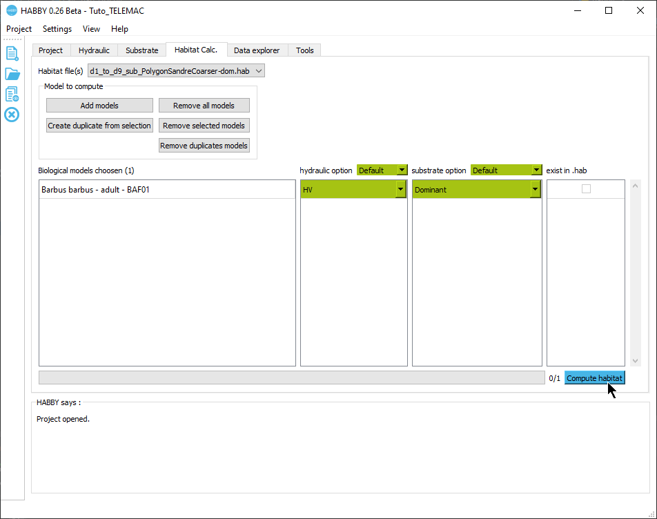
- Open the tab <hi #9BFFFF>Calc. Habitat</hi> tab.
- Check for <hi #9BFFFF>Habitat File(s)</hi> that the 'd1_to_d9_sub_PolygonSandreCoarser-dom.hab' file is selected.
- To add biological models to be calculated, click on the <hi #9BFFFF>[Add Models]</hi> button.
This opens the biological model explorer.
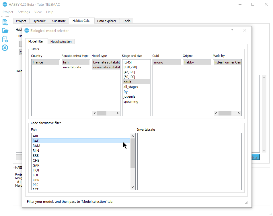
- In the first tab <hi #9BFFFF>Model filter</hi>, refine your search by the following criteria:
- <hi #9BFFFF>Country</hi>: 'France'.
- <hi #9BFFFF>Aquatic animal type</hi>: 'fish'.
- <hi #9BFFFF>Stage and size</hi>: 'adult'.
- <hi #9BFFFF>Code alternative filter</hi> : 'BAF'.
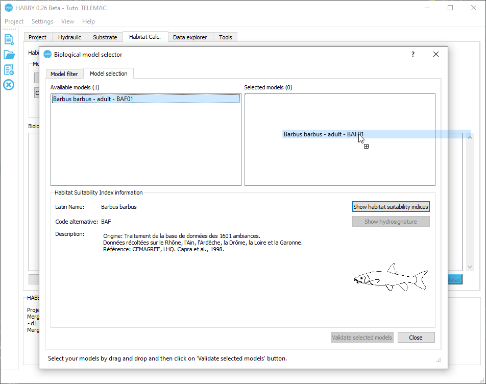
- In the second tab <hi #9BFFFF>Model selection</hi>:
- Click on the model 'Barbus barbus - adult - BAF01' in the left-hand list <hi #9BFFFF>Available models</hi>.
- (Optional) You can click on <hi #9BFFFF>[Show habitat suitability indices]</hi> to display the biological model in an interactive figure
- Drag and drop from left to right the 'Barbus barbus - adult - BAF01' model into the right-hand list <hi #9BFFFF>Selected models</hi>.
- Validate with the <hi #9BFFFF>[Validate selected models]</hi> button.
The model 'Barbus barbus - adult - BAF01' has been added to the list of models to be calculated.
- The hydraulics and substrate options for the biological model 'Barbus barbus - adult - BAF01' are left as default:
- <hi #9BFFFF>Hydraulic option</hi>: 'HV' (Height and Velocity).
- <hi #9BFFFF>Substrate option</hi>: 'Dominant' (Dominant substrate).
- You can now start the habitat calculation for the adult barbel with the <hi #47B5E6>[Compute habitat]</hi> button.
Once the process is finished, the result of the model 'BAF01_adult_HV_Dominant' has been added to the file 'd1_to_d9_sub_PolygonSandreCoarser-dom.hab'. By default, at each calculation, the text habitat calculation result file is created: 'd1_to_d9_sub_PolygonSandreCoarser-dom_spu.txt' describing the habitat values and the weighted usable area of adult barbel for each simulated discharge.
You can view the results in detail, either via the figures or via exports from the explorateur de données.
The *User guide: Calculating habitat from a .hab file explains in more detail the possibilities offered by HABBY.
Visualising habitat results
Preamble
In this tutorial, for the adult barbel, we will :
- Create figures to visualise:
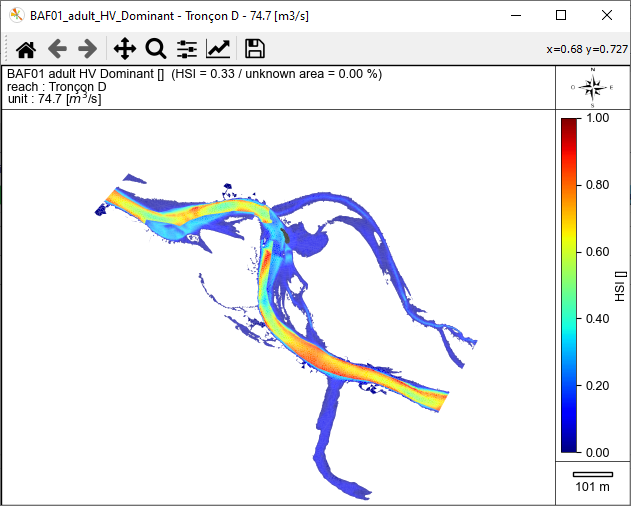
- an interactive habitat map for a discharge of 74.7 m3/s.
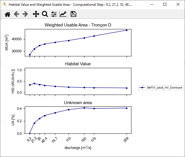
- an interactive habitat record for all discharges.
- Create GIS, 3D and TXT file exports.
- View the exported files:
- GIS representing the mesh for all discharges (.gpkg).
- 3D representing the topography of the river bottom (.stl).
- 3D representing the water level for all discharges (.pvd representing several .vtu).
- TXT describing the state of the mesh for all discharges.
To view the data in detail as a figure and as a file export:
- Open the <hi #9BFFFF>Data Explorer</hi> tab.
Figures
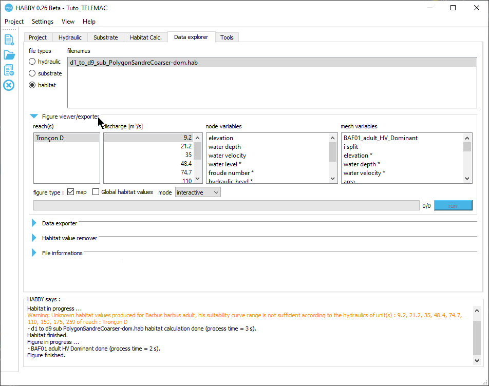
- In the <hi #9BFFFF>Data Explorer</hi> tab, for <hi #9BFFFF>file types</hi>, select 'habitat'.
- In the list of <hi #9BFFFF>File name</hi>, select the file 'd1_to_d9_sub_PolygonSandreCoarser-dom.hab'.
- Open the group <hi #9BFFFF>Figure viewer/exporter</hi> by clicking on its name.
Interactive map
- In this group <hi #9BFFFF>Figure viewer/explorer</hi>, choose:
- <hi #9BFFFF>reach(s)</hi>: 'Tronçon D'.
- <hi #9BFFFF>discharge [m3/s]</hi>: '74.7'.
- <hi #9BFFFF>mesh variables</hi>: 'BAF01_adult_HV_Dominant'.
- Figure options:
- <hi #9BFFFF>map</hi>: enabled.
- <hi #9BFFFF>global habitat value</hi>: disabled.
- <hi #9BFFFF>mode</hi>: 'interactive'.
- Start the figure creation process with the <hi #47B5E6>[run]</hi> button.
An interactive habitat map is then displayed.
NB: To close all interactive figure windows, use the ![]() button in the main window's quick menu.
button in the main window's quick menu.
Interactive Chronicle
- In this group <hi #9BFFFF>Figure viewer/exporter</hi>, choose:
- <hi #9BFFFF>tronçon(s)</hi>: 'Tronçon D'.
- <hi #9BFFFF>discharge [m3/s]</hi></hi>: all discharges (from '9.2' to '259').
- <hi #9BFFFF>mesh variables</hi>: 'BAF01_adult_HV_Dominant'.
- Figure options:
- <hi #9BFFFF>map</hi>: disabled.
- <hi #9BFFFF>global habitat value</hi>: enabled.
- <hi #9BFFFF>mode</hi>: 'interactive'.
- Start the figure creation process with the <hi #47B5E6>[run]</hi> button.
An interactive habitat chronicle is then displayed.
NB: To close all interactive figure windows, use the ![]() button in the main window's quick menu.
button in the main window's quick menu.
Exports
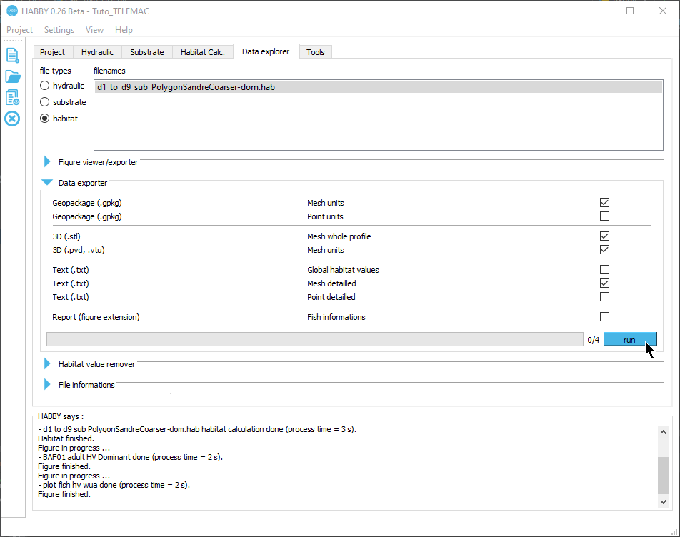
In the <hi #9BFFFF>Data Explorer</hi> tab, for <hi #9BFFFF>file types</hi>, check that 'habitat' is selected.
- In the list of <hi #9BFFFF>File name</hi>, check that the file 'd1_to_d9_sub_PolygonSandreCoarser-dom.hab' is selected.
- Preferably, close the <hi #9BFFFF>Figure viewer/exporter</hi> group.
- Open the group <hi #9BFFFF>Data exporter</hi> by clicking on its name.
- Check the following items:
- <hi #9BFFFF>Geopackage (.gpkg) Mesh units</hi>
- <hi #9BFFFF>3D (.slt) Mesh whole profile</hi> (DEM)
- <hi #9BFFFF>3D (.pvd, .vtu) Mesh units</hi>
- <hi #9BFFFF>TXT (.txt) Mesh detailled</hi>
- Start the export process with the <hi #47B5E6>[run]</hi> button.
At the end of the process, all the requested files have been exported.
NB: All exported files are located in the project's output directory. To access them, use the ![]() button in the main window's quick menu.
button in the main window's quick menu.
SIG
First, we will look at the exports <hi #9BFFFF>Geopackage (.gpkg) Mesh units</hi>, which is the file 'd1_to_d9_sub_PolygonSandreCoarser-dom_Troncon D_mesh.gpkg'.
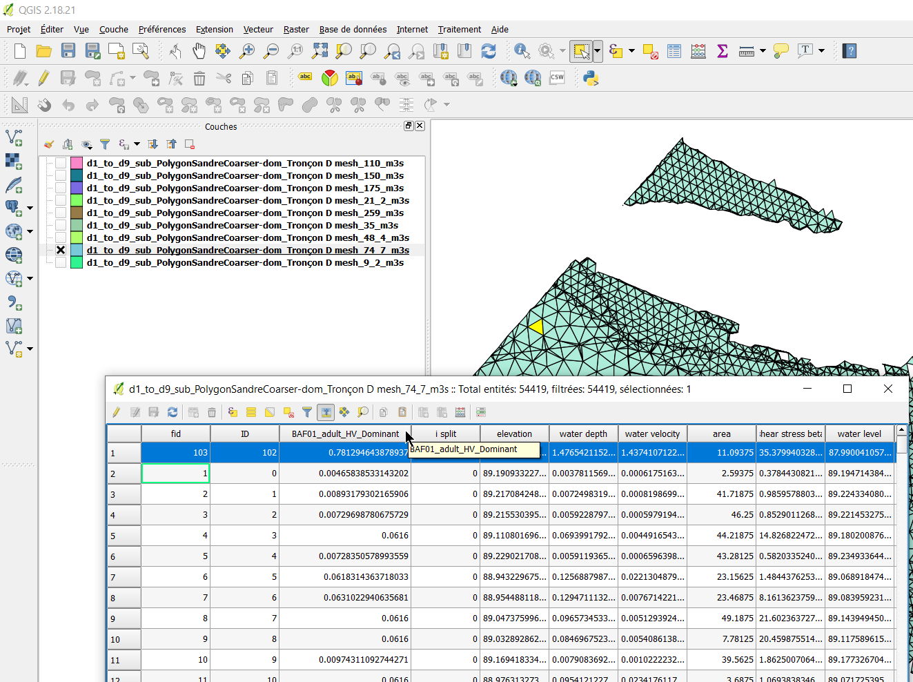
- Open this file 'd1_to_d9_sub_PolygonSandreCoarser-dom_Troncon D_mesh.gpkg' in the project directory ('…\Tuto_TELEMAC\output\GIS') in your GIS software.
This Geopackage file contains several layers (each equivalent to a Shapefile) of triangular polygons (mesh data) for each discharge.
The attribute tables of these layers contain all the mesh data including the habitat data of the adult barbel.
3D
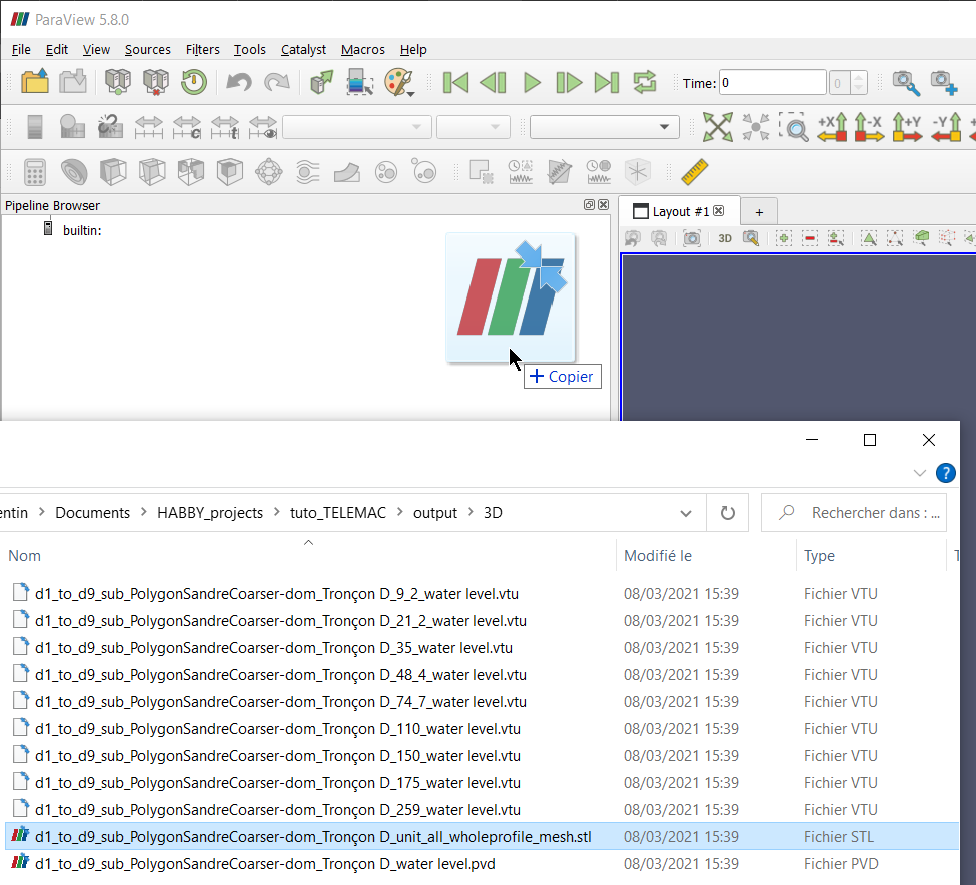
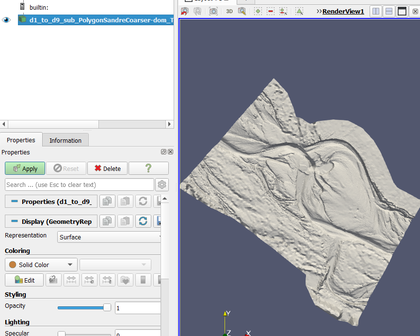
In a second step, we will look at the exports <hi #9BFFFF>3D (.stl) Mesh whole profile</hi>, i.e. the file 'd1_to_d9_sub_PolygonSandreCoarser-dom_Troncon D_unit_all_wholeprofile_mesh.stl'. This 3D .stl (stereolithography) file represents the digital terrain model of the watercourse in 3 dimensions.
- Open this file in the project directory ('…\Tuto_TELEMAC\output3D') in the Paraview software, using drag and drop.
In a third step, we will look at the exports <hi #9BFFFF>3D (.pvd, .vtu) Mesh units</hi>, namely:
- the file 'd1_to_d9_sub_PolygonSandreCoarser-dom_Troncon D_water level.pvd'.
- the 'd1_to_d9_sub_PolygonSandreCoarser-dom_Troncon D_XXXX_water level.vtu' files.
Together, these 3D .pvd and .vtu files represent the water level in 3 dimensions for each unit.
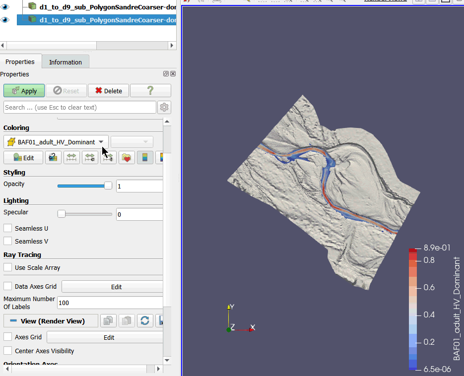
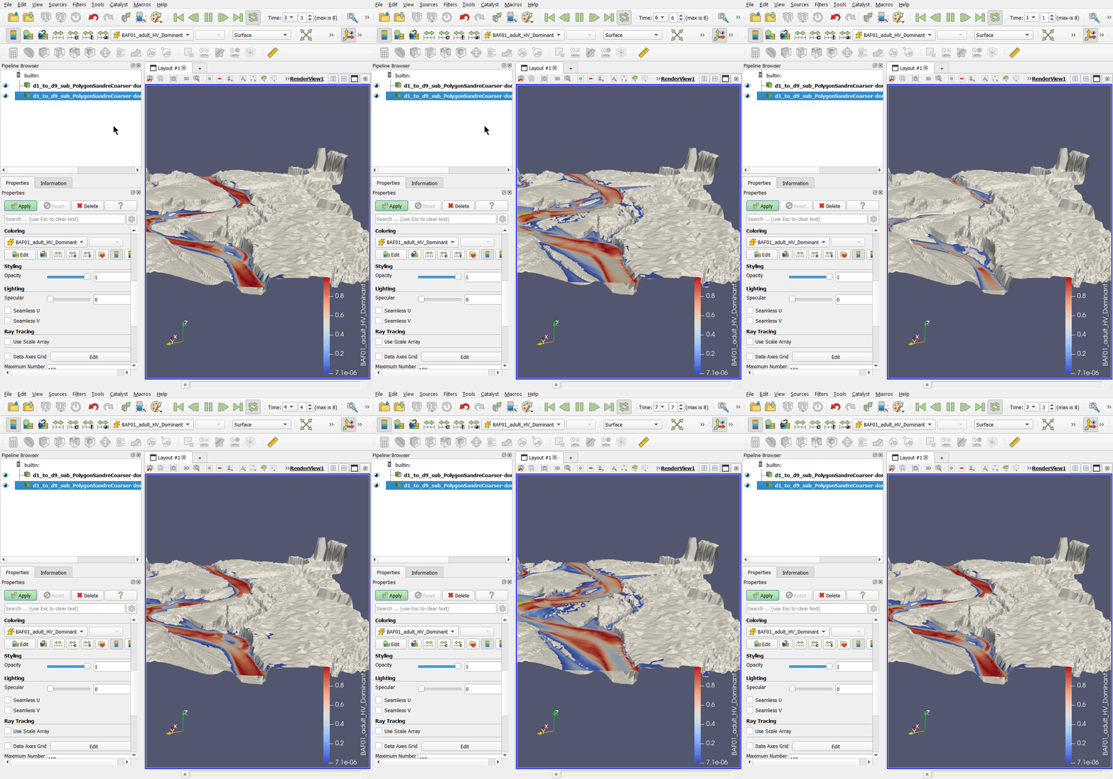
- Add the file 'd1_to_d9_sub_PolygonSandreCoarser-dom_Troncon D_water level.pvd' to the Paraview software, using drag and drop.
- In the 'Properties' tab and then the 'Display' sub-tab of the .pvd file layer, choose for 'Coloring': 'BAF01_adult_HV_Dominant' to display the coloration of the Barbel habitat.
- You can change the angle of view using the mouse or mouse + CTRL
TXT
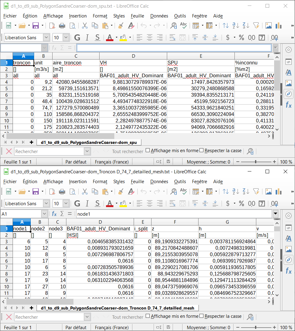
Finally, we will look at the TXT exports in the '…\Tuto_TELEMAC\outputtext' project directory, i.e. :
- 'd1_to_d9_sub_PolygonSandreCoarser-dom_spu.txt': habitat chronicle exported at each calculation.
- 'd1_to_d9_sub_PolygonSandreCoarser-dom_Troncon D_XXXX_detailled_mesh.txt': mesh data per unit, exported manually.
These can be directly used in a spreadsheet by drag and drop.
Using the interpolation tool
Preamble
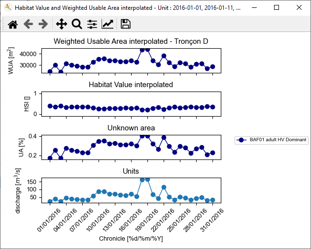
The objective of this last part of the tutorial is to find out the habitat values for a discharge time series using the Interpolation tool.
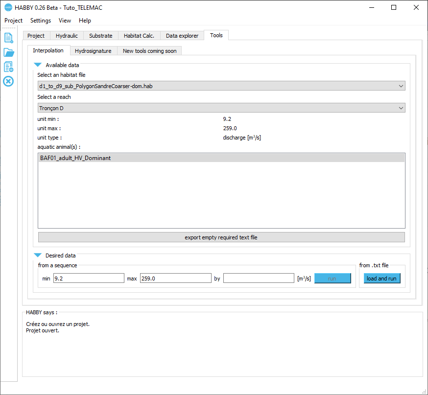
- Open the <hi #9BFFFF>Tools</hi> tab.
- Open the <hi #9BFFFF>Interpolation</hi> sub-tab.
Available data
- If necessary, click on the <hi #9BFFFF>Available data</hi> group to open it.
- Select the habitat file 'd1_to_d9_sub_PolygonSandreCoarser-dom.hab'.
- Check that the 'Tronçon D' is selected.
- Check that the 'BAF01_adult_HV_Dominant' is selected.
The <hi #9BFFFF>Desired data</hi> group is then ready to choose the data to be interpolated.
Desired data
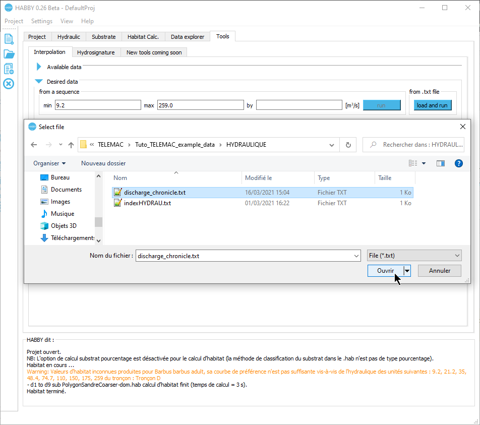
- If necessary, close the <hi #9BFFFF>Data available</hi> group.
- If necessary, click on the <hi #9BFFFF>Desired data</hi> group to open it.
- Select the discharge chronicle file 'discharge_chronicle.txt' with the <hi #47B5E6>[load and run]</hi> button of the group <hi #9BFFFF>from .txt file</hi>.
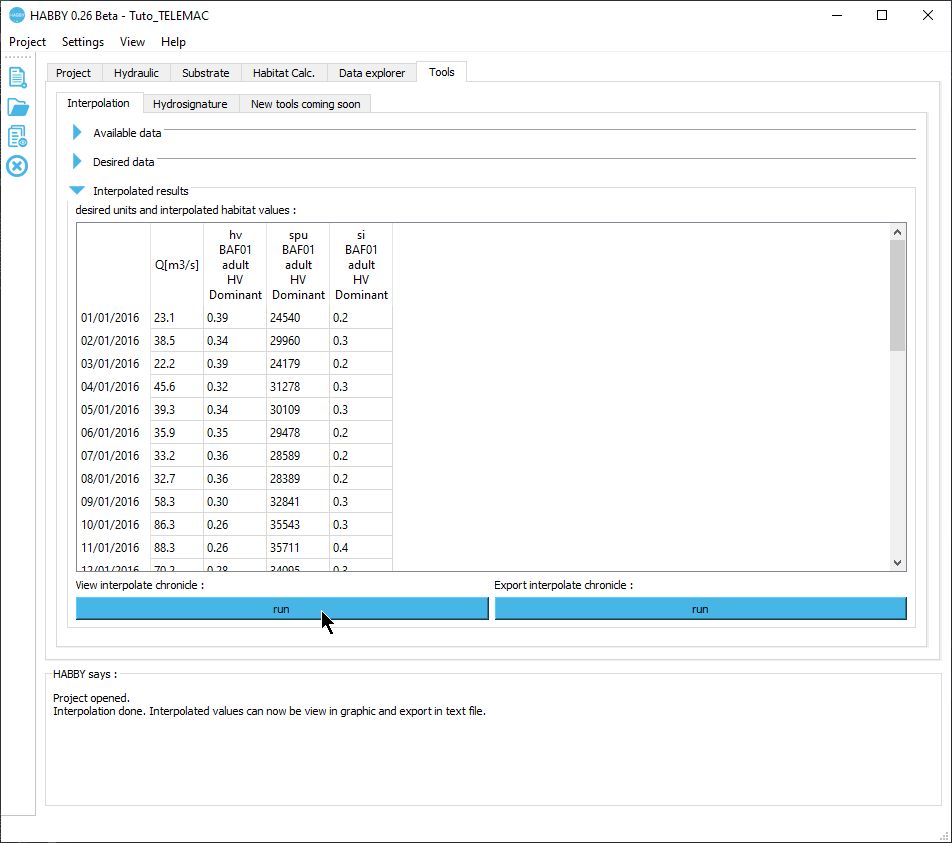
The interpolated results are then displayed in the <hi #9BFFFF>Interpolated results</hi> group.
